predict Metrics Operator
The predict operator takes a single time series metric to predict future values. Predicting metrics such as CPU Usage or memory consumption can be useful for resource and capacity planning use cases.
predict supports linear regression (linear) models, which use a linear model on the timestamp to extrapolate into the future, and Auto-regressive (ar) models, which use a window of previously observed data to predict future values. Note that prediction using an AR model does not output any predictions in the first time window.
The predict operator outputs two time series: the original input time series and the predicted time series that extends into the future. The predicted time series is also depicted over a portion of the historical time range so that the user can validate forecast accuracy at a glance against actual values.
Syntax
predict [model=<model>] [forecast=<forecast>] [ar.window=<ar.window>]
Where:
modelspecifies the type of regression you want to perform:- linear—use the linear regression model. This is the default value if
modelis not specified. - ar—use the auto-regression model.
- linear—use the linear regression model. This is the default value if
forecastspecifies how far into the future you want to forecast.- You can specify
forecastin either in data points or in seconds (s), minutes (m), or hours (h). If no unit of time is specified, the value is interpreted as data points. - The default
forecastvalue is 3 data points. - The maximum value of
forecastyou should set depends on the quantization for your query. If your data is quantized to seconds,forecastmust be less than 50s. If your data is quantized to minutes,forecastmust be less than 50m.
- You can specify
ar.windowis an integer value that specifies how many past data points to use in the next prediction, whenmodelis set to ar.ar.windowmust be less than 50% of all data points gathered by the metrics query. If no value is specified, the system uses 20% of the query time range as thear.window.
Limitations
- Currently, we only support a single time series metric as input.
- The
predictoperator cannot be used in monitors. - We cap forecasts to at most 50 data points in the future. If the
forecastparameter exceeds 50 data points, we give a warning and cap predictions at 50 data points. - The auto-regressive model’s output time series does not depict data points at the beginning of the historical time range.
- At least two data points are required to make predictions for linear regression.
Examples
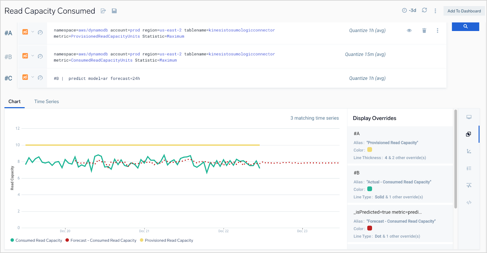
Example 1: Read Capacity Consumed for an AWS DynamoDB Table
In this example, a developer would like to forecast Read Capacity Consumed for an AWS DynamoDB table over the next 24 hours. Series B in the screenshot below provides the input for the actual Read Capacity Consumed time series. Series C takes Series B as input to create a forecast using the auto-regression model 24 hours into the future.
Series B:
namespace=aws/dynamodb account=prod region=us-east-2 tablename=kinesistosumologicconnector metric=ConsumedReadCapacityUnits Statistic=Maximum
Series C:
#B | predict model=ar forecast=24h
The forecast is compared with the Provisioned Read Capacity (Series A) so that the developer can validate if the DynamoDB table has sufficient read capacity to support forecasted read consumption.
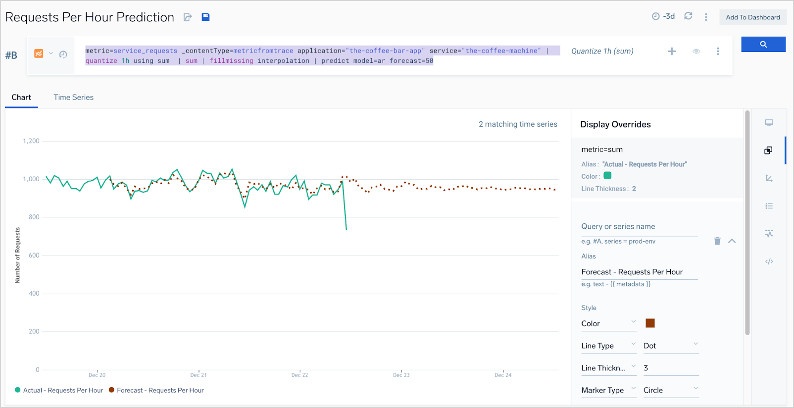
Example 2: Forecast Requests for a Service that Uses Sumo Logic APM
Sumo Logic APM renders golden signals from trace data as request, error, and latency time series. In this example, the developer of the “coffee-bar-app” wants to forecast requests per hour for the “coffee-machine” service using metrics derived from transaction traces. The the auto-regressive model predicts requests per hour 50 data points into the future:
metric=service_requests _contentType=metricfromtrace application="the-coffee-bar-app" service="the-coffee-machine" | quantize 1h using sum | sum | fillmissing interpolation | predict model=ar forecast=50